Plot a Maxwell triangle

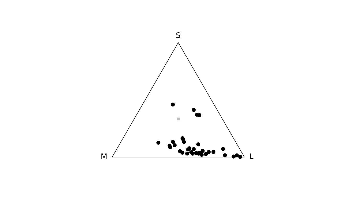
Produces a Maxwell triangle plot.

Usage

triplot(
  tridata,
  labels = TRUE,
  achro = TRUE,
  achrocol = "grey",
  achrosize = 0.8,
  labels.cex = 1,
  out.lwd = 1,
  out.lcol = "black",
  out.lty = 1,
  square = TRUE,
  gamut = FALSE,
  ...
)

Arguments

tridata

(required) a data frame, possibly a result from the colspace() or trispace() function, containing values for the 'x' and 'y' coordinates as columns (labeled as such).

labels

logical. Should the name of each cone be printed next to the corresponding vertex?

achro

should a point be plotted at the origin (defaults to TRUE)?

achrocol

color of the point at the origin achro = TRUE (defaults to 'grey').

achrosize

size of the point at the origin when achro = TRUE (defaults to 0.8).

labels.cex

size of the arrow labels.

out.lwd, out.lcol, out.lty

graphical parameters for the plot outline.

square

logical. Should the aspect ratio of the plot be held to 1:1? (defaults to TRUE).

gamut

logical. Should the polygon showing the possible colours given visual system and illuminant used in the analysis (defaults to FALSE). This option currently only works when qcatch = Qi.

...

additional graphical options. See par().

References

Maxwell JC. (1970). On color vision. In: Macadam, D. L. (ed) Sources of Color Science. Cambridge, MIT Press, 1872 - 1873.

Kelber A, Vorobyev M, Osorio D. (2003). Animal colour vision - behavioural tests and physiological concepts. Biological Reviews, 78, 81 - 118.

MacLeod DIA, Boynton RM. (1979). Chromaticity diagram showing cone excitation by stimuli of equal luminance. Journal of the Optical Society of America, 69, 1183-1186.

Author

Thomas White thomas.white026@gmail.com

Examples

data(flowers)
vis.flowers <- vismodel(flowers, visual = "apis")
tri.flowers <- colspace(vis.flowers, space = "tri")
plot(tri.flowers)