Perceptually-corrected chromaticity diagrams

Plot options for jnd2xyz objects.

jndplot(
  x,
  arrow = c("relative", "absolute", "none"),
  achro = FALSE,
  arrow.labels = TRUE,
  arrow.col = "darkgrey",
  arrow.p = 1,
  labels.cex = 1,
  margin = "recommended",
  square = TRUE,
  ...
)

Arguments

x: (required) the output from a jnd2xyz() call.
arrow: If and how arrows indicating receptor vectors should be drawn. Options are "relative" (default), "absolute" or "none". See description.
achro: Logical. Should the achromatic variable be plotted as a dimension? (only available for dichromats and trichromats, defaults to FALSE).
arrow.labels: Logical. Should labels be plotted for receptor arrows? (defaults to TRUE)
arrow.col: color of the arrows and labels.
arrow.p: scaling factor for arrows.
labels.cex: size of the arrow labels.
margin: accepts either "recommended", where the function will choose margin attributes, or a numerical vector of the form c(bottom, left, top, right) which gives the number of lines of margin to be specified on the four sides of the plot. (Default varies depending on plot dimensionality).
square: logical. Should the aspect ratio of the plot be held to 1:1? (defaults to TRUE).
...: additional parameters to be passed to plot(), arrows() and graphics::persp() (for 3D plots).

Value

Creates a plot, details of the plot depend on the input data.

Note

the arrow argument accepts three options:

"relative": With this option, arrows will be made relative to the data. Arrows will be centered on the data centroid, and will have an arbitrary length of half the average pairwise distance between points, which can be scaled with the arrow.p argument.
"absolute": With this option, arrows will be made to reflect the visual system underlying the data. Arrows will be centered on the achromatic point in colourspace, and will have length equal to the distance to a monochromatic point (i.e. a colour that stimulates approximately 99.9% of that receptor alone). Arrows can still be scaled using the arrow.p argument, in which case they cannot be interpreted as described.
"none": no arrows will be included.

References

Pike, T.W. (2012). Preserving perceptual distances in chromaticity diagrams. Behavioral Ecology, 23, 723-728.

Author

Rafael Maia rm72@zips.uakron.edu

Examples

# Load floral reflectance spectra
data(flowers)

# Estimate quantum catches visual phenotype of a Blue Tit
vis.flowers <- vismodel(flowers, visual = "bluetit")

# Estimate noise-weighted colour distances between all flowers
cd.flowers <- coldist(vis.flowers)
#> Quantum catch are relative, distances may not be meaningful
#> Calculating noise-weighted Euclidean distances

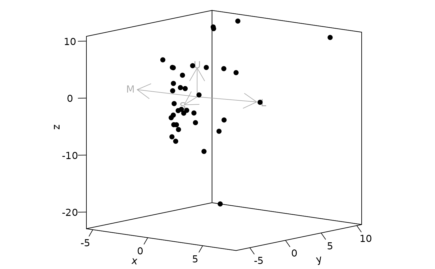
# Convert points to Cartesian coordinates in which Euclidean distances are
# noise-weighted.
propxyz <- jnd2xyz(cd.flowers)

# Plot the floral spectra in 'noise-corrected' space
plot(propxyz)